This article is still under construction. The final version will be released in the near future.
Abstract
This study presents a design method for a brushless DC (BLDC) motor gimbal system that employs a proportional-integral-derivative (PID) control algorithm for target tracking. The system consists of a 2804-100kv BLDC motor, an AS5600 magnetic encoder, and an ESP32 microcontroller, and is integrated with an industrial camera and a PC for target recognition. The system exhibits adaptability, accuracy, and efficiency. The basic structure and control principles of the gimbal system are initially introduced, followed by a system identification procedure that utilizes the system’s response to a sinusoidal signal. The results obtained from modeling, simulation, and experiments are analyzed and discussed.
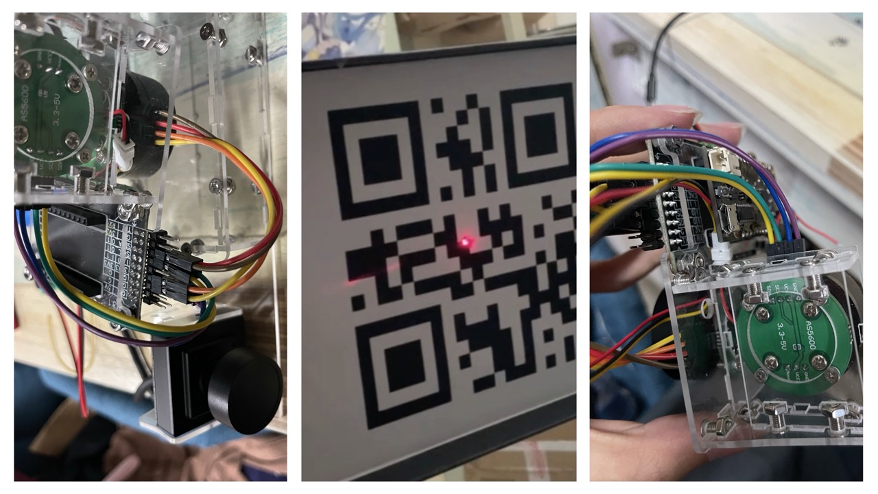
In the experiment, the gimbal system was programmed to track a two-dimensional barcode held by a person, and the accuracy and response speed of the tracking were determined based on a red dot laser emitter fitted onto the gimbal. The experimental results demonstrate that employing the PID control algorithm enables the BLDC gimbal system to accomplish precise target tracking and stable control. This study provides a reference for designing and implementing BLDC motor gimbal systems, and is of practical significance for industrial applications.
Control System Design
To achieve accurate target tracking by PID, the gimbal system must first be modeled. The system consists of two axes: the P-axis, which rotates vertically, and the Y-axis, which rotates horizontally. The P-axis is responsible for controlling the gimbal’s pitch angle, while the Y-axis controls the yaw angle.
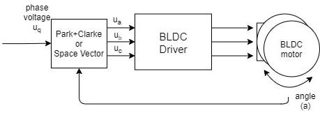
For the P-axis in particular, it can rotate freely without the laser emitter attached, so an open-loop control test—applying voltage as shown in Fig below can be performed directly on the motor. The input is voltage and the output is angular velocity, which aligns with the aforementioned transfer function.
Due to the cable constraints on the Y-axis, it cannot rotate freely. Therefore, the motor is first configured into a cascaded PID closed-loop system, with the feedback channel gain uniformly set to 1. The inner loop uses a velocity control loop with parameters identical to those of the P-axis, while the outer loop employs an angular control loop with a proportional gain of 1 and integral and derivative gains set to 0. This configuration is used to measure the frequency characteristics, with the input being the desired angle and the output being the actual angle.
Since the design steps for the P-axis and Y-axis are largely similar, this paper will use the P-axis as an example to detail the design steps. The Y-axis design will not be repeated here, and only the final design results will be presented.
Sine Wave Response Data Collection and Preprocessing
Before designing the PID control algorithm, the system’s parameters must be identified. To achieve this, the system’s response to a sinusoidal signal is recorded and analyzed. The system’s response is characterized by its magnitude and phase shift, which are used to determine the system’s frequency characteristics.
For the P-axis, we modified the motor control program on the ESP32 to generate sine wave input signals and record the motor’s velocity response. The implementation process is as follows:
Sine Wave Input Generation:
The ESP32 uses its internal clock signal to calculate the standard sine wave value at a given frequency for the current timestamp. This calculated value serves as the reference voltage input to the FOC (Field-Oriented Control) program.Data Recording:
At each timestamp, the ESP32 records:- The motor’s velocity response.
- The corresponding timestamp value.
These values are stored in the ESP32’s internal memory buffer. Once the buffer is full, the entire segment of data is transmitted back to the host computer.
Host-Side Data Reconstruction:
Upon receiving the complete data from the ESP32, the host computer reconstructs the input voltage signal using the same sine wave algorithm based on the recorded timestamps. This results in two sets of data points:- One set represents the reconstructed input voltage.
- The other set represents the motor’s velocity response.
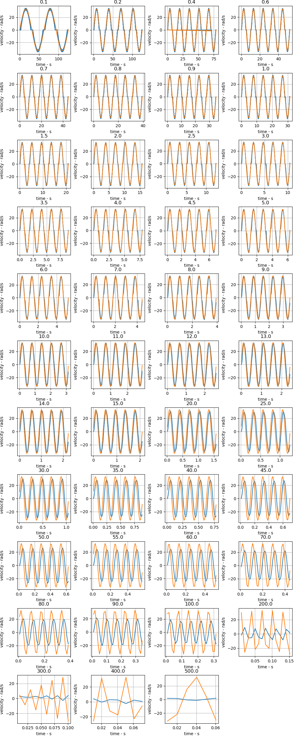
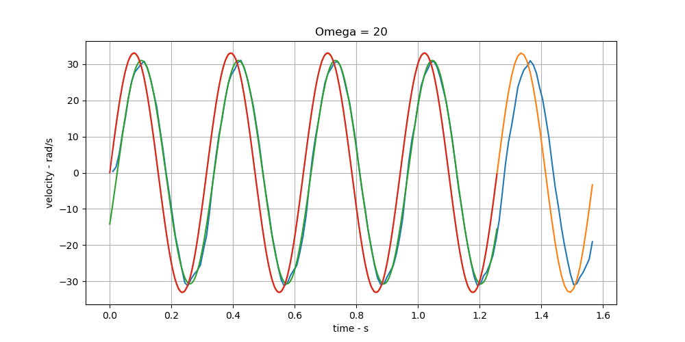
An example of these signals is shown in Fig below, where the orange curve represents the reconstructed input signal, and the blue curve represents the motor’s velocity response.
Memory Optimization:
This approach was chosen due to the limited runtime memory available on the ESP32. Storing both input and output values simultaneously (as floating-point data) would quickly exhaust the available memory. Instead, only the timestamps (stored as unsigned integers) are recorded, significantly reducing memory usage.
This efficient method ensures that the ESP32 can handle the data recording task without exceeding its memory capacity while maintaining the integrity of the collected data for system identification.
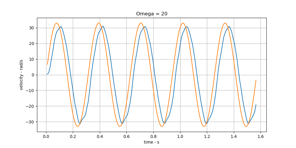
Since the frequency response of the system must inherently correspond to a sinusoidal signal with the same frequency as the input, the parameters of the sinusoidal signals are identified using the least squares method. This approach provides a more intuitive way to derive the frequency characteristics.
The results are shown in Fig below, where:
- The red curve represents the fitted input signal (corresponding to the orange signal).
- The green curve represents the fitted response signal (corresponding to the blue signal).
By fitting the input and output signals to sinusoidal functions, the amplitude, phase shift, and frequency characteristics are directly obtained, facilitating the analysis of the system’s dynamic behavior.
Using the amplitude ratio and phase difference between the two signals, the system’s magnitude-frequency and phase-frequency characteristics can be calculated. From these, the real-frequency and imaginary-frequency characteristics of the system are further derived. However, due to the nature of the parameter identification algorithm, when the signal’s phase lag exceeds 90 degrees, it is misidentified as a lead signal. To address this, the phase of the lead signal is adjusted backward by 180 degrees before proceeding with calculations.
Due to the limitations of the microcontroller’s memory capacity and clock frequency, the sampled signals become nearly unusable when the input signal frequency is too high. Therefore, the input signal frequency range is ultimately set between 0.1 rad/s and 200 rad/s. To optimize the workload, smaller frequency intervals are used for the low-frequency range, while larger intervals are applied in the high-frequency range.

Due to the lack of an external clock source in the experimental setup, it was not possible to achieve a truly fixed sampling time. To address this, the sampling times were calculated by taking the pairwise differences of consecutive timestamp values and averaging them.
The computed average sampling time is
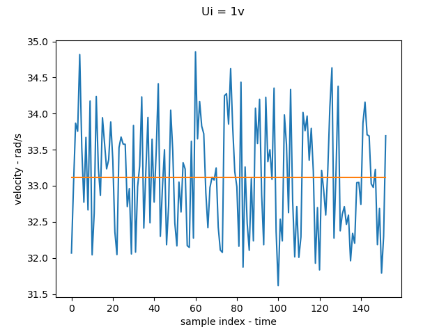
The amplitude of the input signal was determined by applying a fixed voltage to the motor and allowing it to reach steady-state operation. During the steady state, a segment of the motor’s velocity output was sampled, and the average velocity was calculated. The result,
Finally, the obtained real and imaginary frequency data were imported into Matlab to generate the system’s Bode plot for initial validation. The resulting plot is shown in Fig below.

The complete dataset and the data processing program can be found in the appendix.
BLDC Motor System Identification Design
After collecting the system’s frequency response data, the next step is to identify the system’s dynamic, which also known as system modeling.
According to the work of Shamseldin and Abdelbar M, the BLCD motor can be modeled as a second-order system, expressed as
However, measuring parameters such as the viscous friction coefficient and moment of inertia is quite challenging. So we decided to use Matlab’s System Identification Toolbox to determine the unknown parameters in this transfer function.
First, the system’s frequency characteristics are imported into the Matlab workspace. Then, the System Identification Toolbox is launched. The previously measured frequency response data is loaded into the toolbox, and a transfer function model is selected. The number of poles and zeros is specified based on the system’s characteristics.
As discussed earlier, the BLDC motor’s transfer function, when ignoring the load, is expected to have two poles and no zeros. However, practical results showed that this model achieves a maximum fit of only 70.71% with the measured frequency response data. To achieve a higher fit, the load must be considered. Therefore, the system is modeled as a discrete system with two poles and one zero for system identification.
The final identified transfer function is shown in Equation below, with a fit of 85.72%:
PID Controloer Design
Based on the transfer function obtained earlier, a Simulink model is constructed. Using MATLAB’s PID Tuner, the velocity loop PID controller parameters are determined as follows:
- ( P = 0.107 )
- ( I = 10.58 )
- ( D = 0.0002708 )
These parameters are then entered into Simulink, and further tuning is conducted to finalize the velocity loop PID parameters.
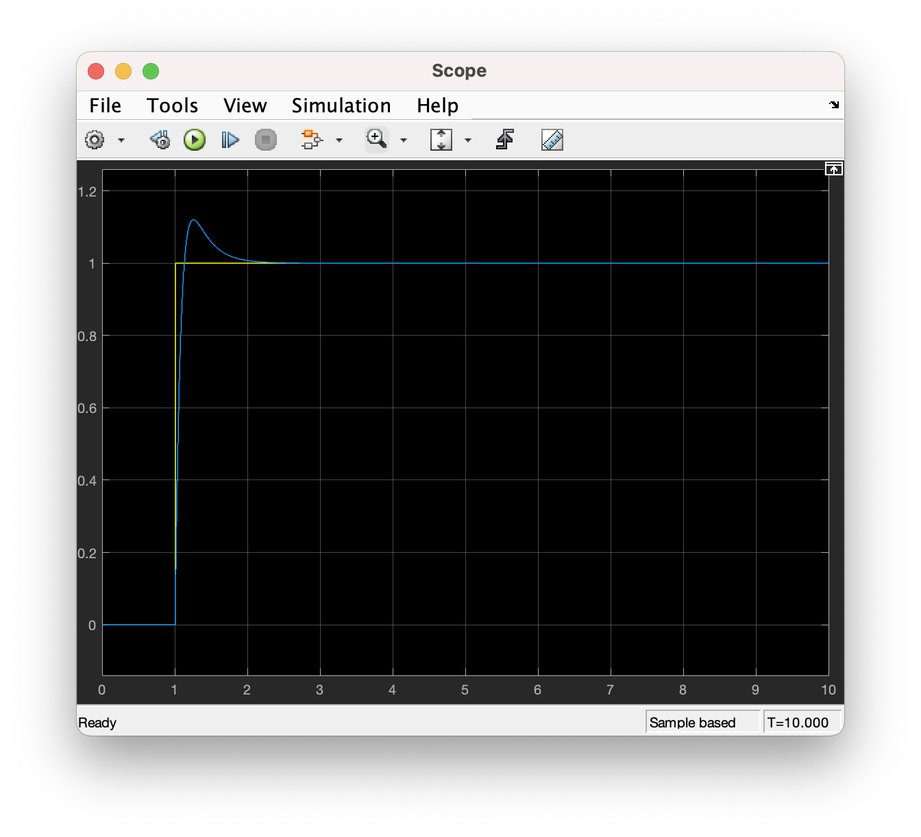
Next, the tuning functionality of Simulink’s PID module is used to determine the angle loop parameters. Similar to MATLAB’s PID Tuner, the interface provides slider controls to adjust the desired system response characteristics, with the step response displayed in real-time for reference. Once the desired response is achieved, clicking the “Update Block” button automatically applies the tuned parameters to the Simulink model. The final PID controller parameters for the angle loop are:
- ( P = 21.42 )
- ( I = 51.6 )
- ( D = 1.492 )
And the simulation for step response is shown in Fig below.
The obtained parameters are entered into the ESP32 control program, and the final unit step response of the system is shown in Fig below.
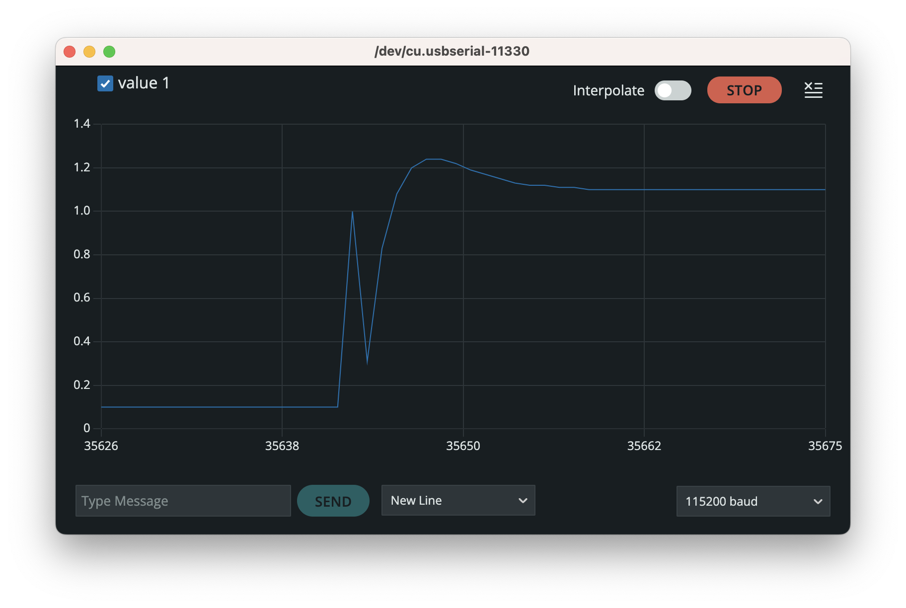
The error of approximately 0.1 is actually due to the structural installation compensation mentioned earlier, rather than a steady-state error from the control system. The spike during the rising phase of the data is caused by sensor noise.
It can be observed that the actual system response closely matches the simulated response after implementing the simulation parameters in the physical system. This consistency validates the effectiveness of the system identification and controller design.
Structural Description
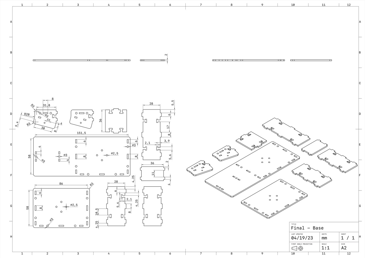
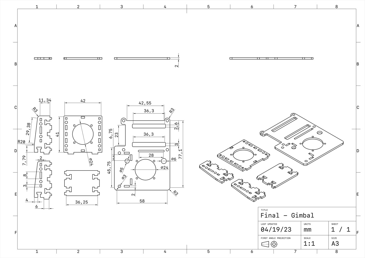
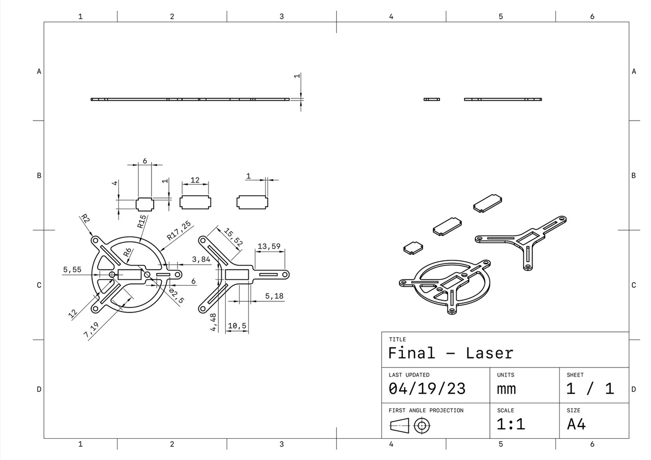
Due to budget constraints, we were unable to purchase a slip ring for transmitting control data. As a result, the Y-axis motor is mounted in reverse, with the main controller and motor driver also located on the Y-axis. This configuration prevents excessive Y-axis rotation during debugging, thereby avoiding potential damage to the motor cables should the gimbal malfunction. Additionally, to prevent the industrial camera cables from interfering with the gimbal’s motion, the camera is fixed to the base, maintaining a constant relative position to the gimbal.
Appendix
